From RNA-seq to chemical enrichment: a complete workflow

Biological context

Dexamethasone is a synthetic glucocorticoid widely used as an anti-inflammatory and immunosuppressive agent. Its transcriptomic effects on immune cells are well characterised: it suppresses pro-inflammatory cytokines, reprograms monocyte and lymphocyte gene programmes, and leaves a distinctive signature in peripheral blood mononuclear cells (PBMCs).

This tutorial asks a straightforward question: given the RNA-seq signature of dexamethasone treatment in human PBMCs, which chemicals in the Comparative Toxicogenomics Database (CTD) share that signature?

We answer it using all four methods provided by ctdR — GSEA, ORA, CAMERA, and GSVA — and show how to visualise and interpret each result.

Data source: we use GSE311566, a public GEO series comparing the effects of PFAS chemicals and dexamethasone on human PBMCs from female donors. We work with the Dexamethasone vs. vehicle (DMSO/Ctrl) contrast, female samples only (7 samples total: 4 Ctrl + 3 Dex).

What this tutorial covers

Downloading and preparing public RNA-seq count data from GEO

Differential expression with limma

Chemical enrichment analysis (GSEA, ORA, CAMERA, GSVA) using ctdR

Visualisation with plot_CTD()

What this tutorial does NOT cover

Raw read quality control (FastQC, trimming)

Alignment and count generation

Normalisation strategy selection (TMM, VST, etc.)

Batch correction or covariate adjustment

Biological replicate adequacy or power analysis

This is an end-to-end illustration of the ctdR workflow on publicly available processed data, not a template for a production differential expression pipeline.

Setup

library(ctdR)
library(limma)
library(org.Hs.eg.db)
library(AnnotationDbi)

Step 1 — Download data from GEO

The normalised count matrix for GSE311566 is available directly from NCBI FTP. We download it once and cache it in the session temporary directory; re-running this chunk skips the download if the file already exists.

GEO_URL <- paste0(
    "https://ftp.ncbi.nlm.nih.gov/geo/series/GSE311nnn/GSE311566/",
    "suppl/GSE311566_PBMCs_Female_normalized_counts.txt.gz"
)
tmp_gz <- file.path(tempdir(), "GSE311566_Female_normalized_counts.txt.gz")
if (!file.exists(tmp_gz)) {
    message("Downloading GSE311566 from NCBI FTP ...")
    utils::download.file(GEO_URL, tmp_gz, mode = "wb", quiet = FALSE)
}

Step 2 — Prepare the expression matrix

counts <- utils::read.table(
    gzfile(tmp_gz),
    header = TRUE, sep = "\t", row.names = 1,
    check.names = FALSE, stringsAsFactors = FALSE
)
counts$DESCRIPTION <- NULL  # all NA in this dataset

# Female Ctrl and DEX samples only
keep_cols <- grep("^(Ctrl|DEX)_F_", colnames(counts), value = TRUE)
counts <- counts[, keep_cols]
group <- factor(
    ifelse(grepl("^DEX_", keep_cols), "Dex", "DMSO"),
    levels = c("DMSO", "Dex")
)
message(nrow(counts), " genes, ", ncol(counts), " samples: ",
    paste(table(group), names(table(group)), sep = " ", collapse = " / "))

The GEO file uses Ensembl gene IDs. We strip version suffixes and map to Entrez IDs, which are the identifier type required by ctdR.

ensg <- sub("\\..*$", "", rownames(counts))
entrez_map <- AnnotationDbi::mapIds(
    org.Hs.eg.db,
    keys     = ensg,
    keytype  = "ENSEMBL",
    column   = "ENTREZID",
    multiVals = "first"
)
keep_g <- !is.na(entrez_map) & !duplicated(entrez_map)
counts <- counts[keep_g, ]
rownames(counts) <- entrez_map[keep_g]
expr <- log2(as.matrix(counts) + 1)
message(nrow(expr), " genes retained after Entrez mapping")

Step 3 — Import CTD data

ctd_csv <- "~/Downloads/CTD_chem_gene_ixns.csv"
ctd_gz  <- "~/Downloads/CTD_chem_gene_ixns.csv.gz"

if (file.exists(ctd_csv)) {
    message("Using full CTD: ", ctd_csv)
    import_CTD(ctd_csv)
} else if (file.exists(ctd_gz)) {
    message("Using full CTD (compressed): ", ctd_gz)
    import_CTD(ctd_gz)
} else {
    message(
        "Full CTD not found in ~/Downloads/ — using bundled toy sample ",
        "(10 chemicals). Results will be illustrative only.\n",
        "Download CTD_chem_gene_ixns.csv.gz from ctdbase.org for a ",
        "powered analysis."
    )
    import_CTD(system.file(
        "extdata", "CTD_chem_gene_ixns_sample.csv",
        package = "ctdR"
    ))
}

Note on CTD coverage: this tutorial uses the small toy dataset bundled with ctdR (10 chemicals, 17 genes). It is sufficient to demonstrate the API and visualisations. For a powered analysis capable of discovering novel chemical associations, download the full CTD_chem_gene_ixns.csv.gz from https://ctdbase.org/reports/CTD_chem_gene_ixns.csv.gz and run import_CTD() on that file instead.

Step 4 — Differential expression with limma

We fit a linear model and apply empirical Bayes moderation. The design matrix has two columns: the intercept (DMSO baseline) and groupDex (Dex vs DMSO contrast, coefficient 2).

design <- model.matrix(~ group)
colnames(design)
#> [1] "(Intercept)" "groupDex"

fit <- limma::lmFit(expr, design)
fit <- limma::eBayes(fit)

de <- limma::topTable(fit, coef = 2, n = Inf, sort.by = "P")
de$EntrezID <- rownames(de)

head(de[, c("EntrezID", "logFC", "t", "P.Value", "adj.P.Val")])
#>       EntrezID      logFC         t      P.Value   adj.P.Val
#> 2289      2289  2.8860368  66.81282 5.381612e-09 0.000200056
#> 64744    64744  1.5371202  33.39116 2.148090e-07 0.002665942
#> 8553      8553 -1.2969205 -33.38130 2.151457e-07 0.002665942
#> 8761      8761  0.7060472  27.55983 5.941309e-07 0.005521555
#> 8395      8395 -0.9214413 -25.57857 8.817929e-07 0.006555954
#> 78999    78999  0.9863471  23.27464 1.452352e-06 0.008998287

A brief look at significance:

c(
    total_genes   = nrow(de),
    padj_lt_05    = sum(de$adj.P.Val < 0.05),
    pvalue_lt_05  = sum(de$P.Value  < 0.05)
)
#>  total_genes   padj_lt_05 pvalue_lt_05 
#>        37174          169         4361

Step 5 — Chemical enrichment

GSEA — Gene Set Enrichment Analysis

GSEA uses the full ranked gene list to detect chemicals whose known target genes collectively cluster toward one extreme of the ranking, without requiring a significance threshold. We supply the moderated t-statistic from limma as the stat column so that directionality (up vs down) is preserved and ties at non-significant genes are avoided. Pass nproc = N to parallelise across N cores.

gsea_input <- data.frame(
    EntrezID = de$EntrezID,
    pvalue   = de$P.Value,
    stat     = de$t,       # signed ranking: positive = up in Dex
    row.names = NULL
)
gsea_results <- enrichment_CTD(
    gsea_input, method = "GSEA",
    minSize = 3, maxSize = 500   # gene set size filter
)
head(gsea_results[, c(
    "ChemicalName", "PValue", "PValueAdjusted",
    "NormalizedEnrichmentScore", "FoldEnrichment"
)])
#>       ChemicalName     PValue PValueAdjusted NormalizedEnrichmentScore
#> 1        Estradiol 0.02328381      0.2328381                -1.4470219
#> 2    Acetaminophen 0.74846626      0.9355828                 0.7939608
#> 3   Benzo(a)pyrene 0.71342685      0.9355828                 0.8077455
#> 4          Cadmium 0.73456790      0.9355828                 0.7949407
#> 5        Cisplatin 0.73630832      0.9355828                 0.7844192
#> 6 Cyclophosphamide 0.73809524      0.9355828                -0.8136112
#>   FoldEnrichment
#> 1       33.33723
#> 2       15.17452
#> 3       16.02867
#> 4       16.87423
#> 5       15.08997
#> 6       19.82472

FoldEnrichment here is |ES| / mean(|ES|) across all tested chemicals — a relative measure of how strongly enriched this chemical’s gene set is compared to the average. NES (Normalized Enrichment Score) accounts for gene set size differences and is the primary statistic for ranking chemicals.

plot_CTD(gsea_results, type = "bar", n = 10,
         title = "GSEA — top chemicals by NES")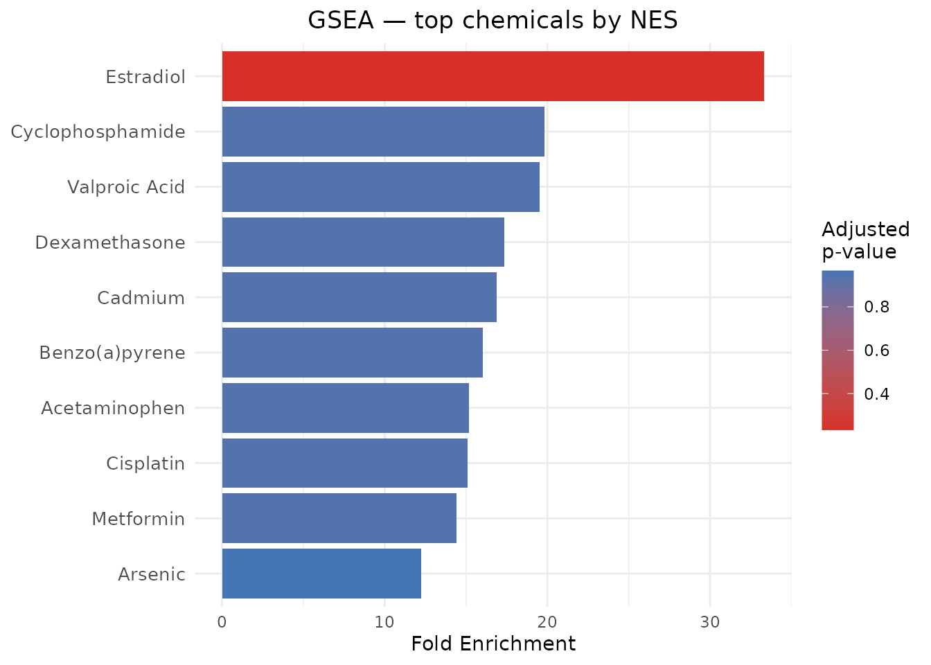

plot_CTD(gsea_results, type = "dot", n = 10,
         title = "GSEA — top chemicals (dot)")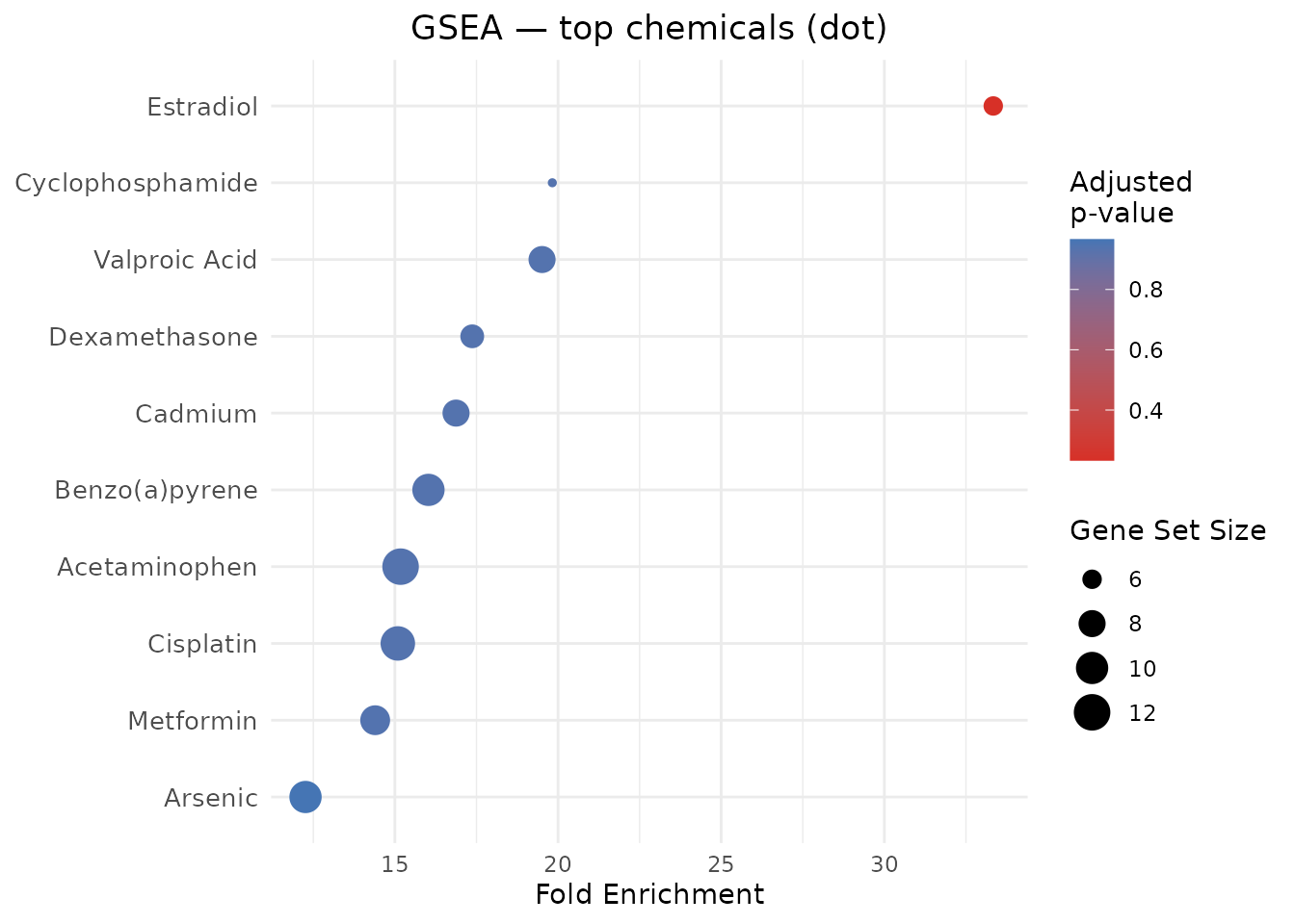

Where is Dexamethasone?

The top-ranked chemical may or may not be Dexamethasone depending on which CTD dataset is loaded. With the full CTD (~11 000 chemicals and strict BH correction) Dexamethasone competes against many other chemicals and may rank lower than expected, or may not reach significance after correction. The code below locates it regardless of its rank:

dex_idx  <- grep("dexamethasone", gsea_results$ChemicalName,
                 ignore.case = TRUE)
if (length(dex_idx) > 0) {
    cat("Dexamethasone: rank", dex_idx, "of", nrow(gsea_results), "\n")
    gsea_results[dex_idx, c("ChemicalName", "PValue", "PValueAdjusted",
                             "NormalizedEnrichmentScore", "FoldEnrichment")]
} else {
    message("Dexamethasone not found — it may be absent from the loaded CTD cache.")
}
#> Dexamethasone: rank 7 of 10
#>    ChemicalName    PValue PValueAdjusted NormalizedEnrichmentScore
#> 7 Dexamethasone 0.7396694      0.9355828                 0.7902494
#>   FoldEnrichment
#> 7       17.37013

Why Dexamethasone may not top the list with the full CTD:

Multiple testing burden — 11 000 tests vs 10 in the toy sample; the BH threshold is ~1 000× more stringent.

Larger gene sets — in the full CTD, Dexamethasone has hundreds of annotated targets; very large sets dilute the GSEA signal in small cohorts (7 samples here).

Competing chemicals — other chemicals may have gene sets that overlap more tightly with the top-ranked DE genes.

Direction-aware GSEA with `interaction_types`

The standard GSEA above uses all CTD interactions regardless of direction. With interaction_types we can restrict each chemical’s gene set to interactions of a specific type, creating a concordance test: do chemicals that are known to increase gene expression share targets with genes we observe up-regulated?

# Chemicals whose INCREASE-expression targets are enriched among up-regulated genes
gsea_up <- enrichment_CTD(
    gsea_input, method = "GSEA",
    minSize = 3, maxSize = 500,
    interaction_types = "increases^expression"
)

# Chemicals whose DECREASE-expression targets are enriched among down-regulated genes
# Flip stat sign so down-regulated genes (negative t) rank at the top
gsea_input_down <- transform(gsea_input, stat = -stat)
gsea_down <- enrichment_CTD(
    gsea_input_down, method = "GSEA",
    minSize = 3, maxSize = 500,
    interaction_types = "decreases^expression"
)

# Chemicals consistent with Dex treatment (up or down, direction-matched)
message("Direction-aware GSEA — increases^expression: ",
        nrow(gsea_up), " chemicals tested")
message("Direction-aware GSEA — decreases^expression: ",
        nrow(gsea_down), " chemicals tested")

A chemical appearing in both gsea_up and gsea_down with positive NES in each is particularly strong evidence of a concordant transcriptomic footprint.

ORA — Over-Representation Analysis

ORA works on a binary gene list: genes declared significant vs the rest of the universe. It asks whether the overlap between your significant genes and each chemical’s known targets is larger than expected by chance (hypergeometric test).

sig <- de[de$adj.P.Val < 0.05, c("EntrezID", "P.Value")]
colnames(sig)[2] <- "pvalue"
message(nrow(sig), " genes at adj.P.Val < 0.05")

ora_results <- enrichment_CTD(
    sig, method = "ORA",
    universe   = de$EntrezID,  # restrict background to measured genes
    minGSSize  = 3,
    maxGSSize  = 500
)

if (nrow(ora_results) > 0) {
    head(ora_results[, c(
        "ChemicalName", "PValue", "PValueAdjusted",
        "FoldEnrichment", "Count", "EnrichedGenes"
    )])
} else {
    message(
        "ORA returned 0 results — expected with the toy CTD sample.\n",
        "Run import_CTD() on the full CTD file for a powered analysis."
    )
}

if (nrow(ora_results) > 0) {
    dex_idx <- grep("dexamethasone", ora_results$ChemicalName,
                    ignore.case = TRUE)
    if (length(dex_idx) > 0) {
        cat("Dexamethasone: rank", dex_idx, "of", nrow(ora_results), "\n")
        ora_results[dex_idx, c("ChemicalName", "PValue", "PValueAdjusted",
                                "FoldEnrichment", "Count")]
    } else {
        message("Dexamethasone not found in ORA results.")
    }
}

plot_CTD(ora_results, type = "dot", n = 10,
         title = "ORA — top chemicals by fold enrichment")

FoldEnrichment in ORA is GeneRatio / BackgroundRatio: the proportion of your significant genes that are targets of this chemical, divided by the same proportion in the background universe. A value greater than 1 indicates over-representation.

CAMERA — Competitive gene-set test

CAMERA tests, for each chemical, whether its target genes show a stronger differential signal than the rest of the transcriptome, while correcting for inter-gene correlation within the gene set. It is particularly well suited to expression matrix experiments with a clear design and contrast.

CAMERA does not consume a pre-computed DEG result: it takes the full expression matrix plus a design and a contrast, and recomputes the differential signal internally. The chemical→gene “index” is built by ctdR from CTD targets. We reuse the design matrix built for limma; here design carries the whole layout while contrast = 2 selects which coefficient to test — the groupDex effect (Dex vs DMSO).

camera_results <- enrichment_CTD(
    expr,
    method   = "CAMERA",
    design   = design,
    contrast = 2
)
head(camera_results[, c(
    "ChemicalName", "PValue", "PValueAdjusted",
    "GeneSetSize", "Direction"
)])
#>     ChemicalName     PValue PValueAdjusted GeneSetSize Direction
#> 1      Estradiol 0.02495925      0.2495925           6      Down
#> 2  Acetaminophen 0.26645058      0.5007785          12        Up
#> 3 Benzo(a)pyrene 0.31813538      0.5007785          10        Up
#> 4        Cadmium 0.16732813      0.5007785           8        Up
#> 5      Cisplatin 0.31687483      0.5007785          11        Up
#> 6  Dexamethasone 0.33074736      0.5007785           7        Up

Unlike ORA and GSEA, CAMERA does not report a FoldEnrichment value — it reports Direction ("Up" or "Down"), indicating whether the chemical’s target genes are predominantly up- or down-regulated under the tested contrast.

plot_CTD(camera_results, type = "bar", n = 10,
         title = "CAMERA — direction-aware chemical enrichment")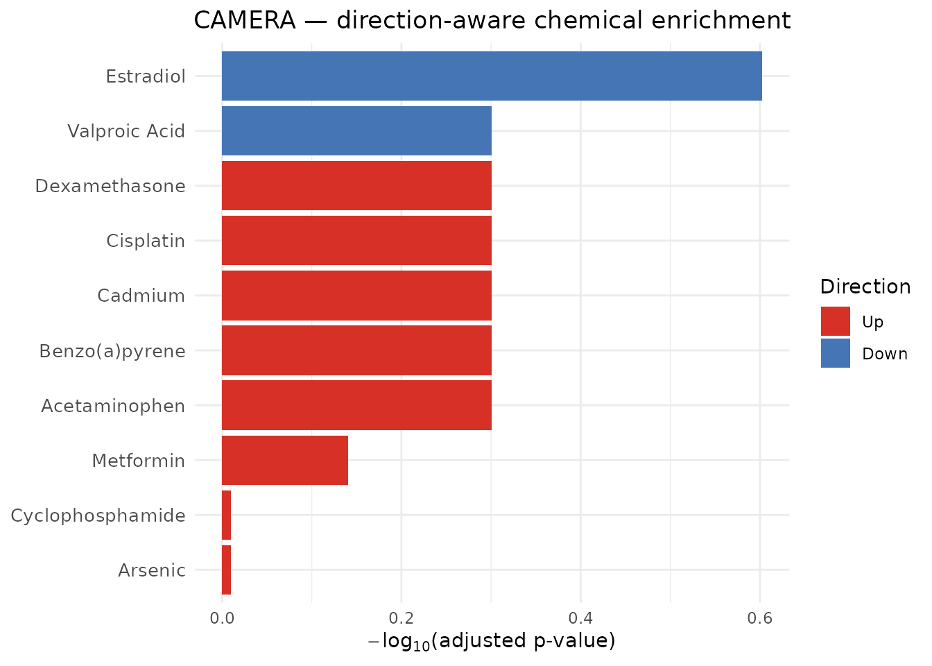

dex_idx <- grep("dexamethasone", camera_results$ChemicalName,
                ignore.case = TRUE)
if (length(dex_idx) > 0) {
    cat("Dexamethasone: rank", dex_idx, "of", nrow(camera_results), "\n")
    camera_results[dex_idx, c("ChemicalName", "PValue", "PValueAdjusted",
                               "GeneSetSize", "Direction")]
} else {
    message("Dexamethasone not found in CAMERA results.")
}
#> Dexamethasone: rank 6 of 10
#>    ChemicalName    PValue PValueAdjusted GeneSetSize Direction
#> 6 Dexamethasone 0.3307474      0.5007785           7        Up

GSVA — Gene Set Variation Analysis

GSVA produces a per-sample enrichment score for each chemical: a matrix with chemicals in rows and samples in columns. There is no single group-level p-value; instead, these scores can be used for clustering, heatmap visualisation, survival association, or as input to downstream tests.

Computation time: GSVA scores all chemicals across all samples. On the full expression matrix this may take a few minutes. Use BiocParallel::register() to speed it up on multi-core machines.

gsva_scores <- enrichment_CTD(
    expr, method = "GSVA",
    minSize = 3, maxSize = 500
)
dim(gsva_scores)  # chemicals x samples
#> [1] 10  7

plot_CTD(gsva_scores,
         title = "GSVA — per-sample chemical enrichment scores")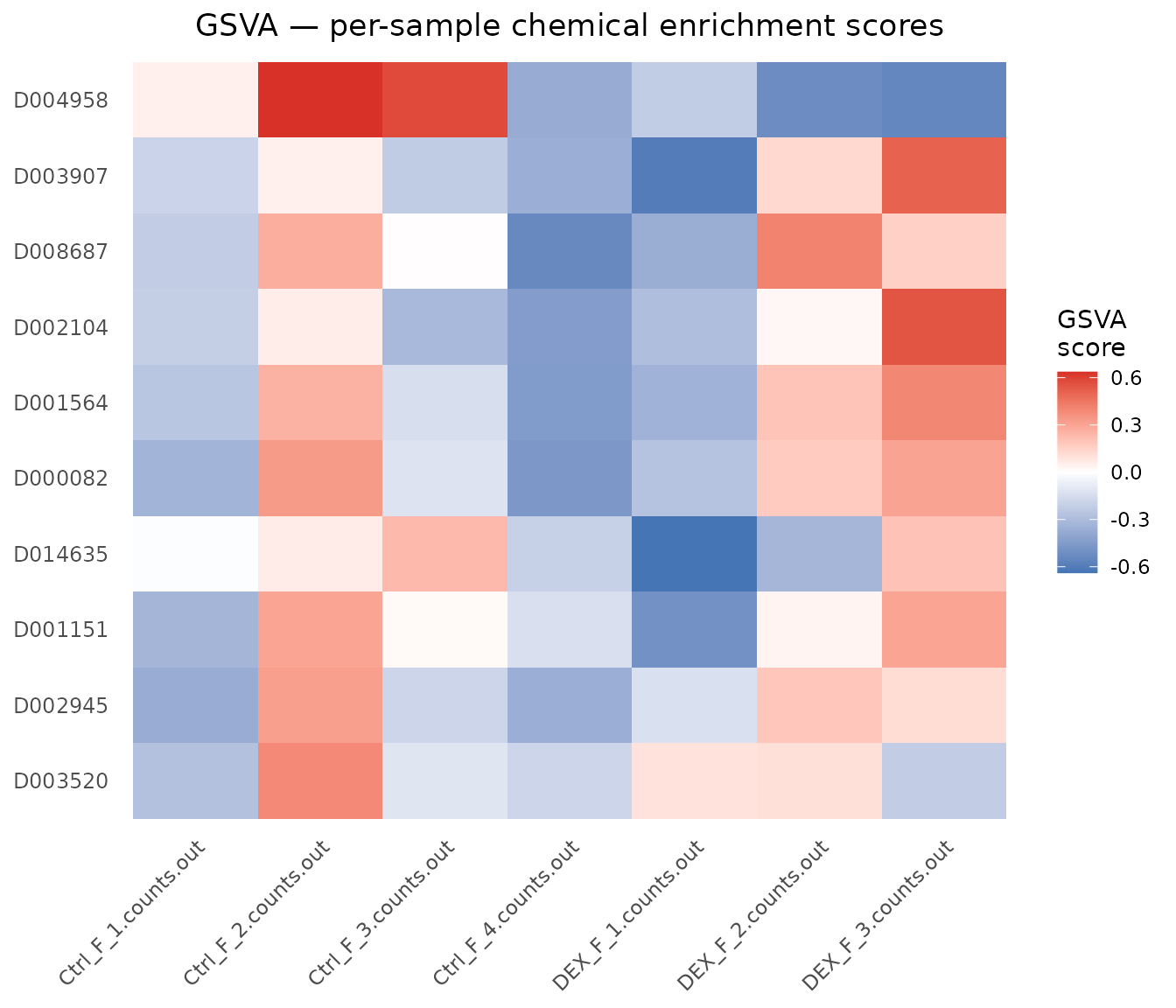

The heatmap rows are chemicals ranked by across-sample variance (top-variance chemicals shown first). Samples that cluster together share a similar chemical-exposure transcriptomic profile.

To inspect Dexamethasone’s per-sample scores directly:

dex_idx <- grep("dexamethasone", rownames(gsva_scores),
                ignore.case = TRUE)
if (length(dex_idx) > 0) {
    cat("Dexamethasone row(s):", rownames(gsva_scores)[dex_idx], "\n")
    gsva_scores[dex_idx, , drop = FALSE]
} else {
    message("Dexamethasone not found in GSVA score matrix.")
}

Positive scores indicate that Dexamethasone’s target genes are collectively up-regulated in that sample relative to the background; negative scores indicate down-regulation. A clear separation between Dex and Ctrl samples (positive scores in Dex, negative in Ctrl, or vice versa) would support the expected glucocorticoid signature.

Step 6 — Comparing results across methods

Each method answers a subtly different question:

Method	Input	Question answered	Key output column
GSEA	Full ranked list	Do this chemical’s targets cluster at the extreme of the ranking?	`NES`, `FoldEnrichment`
ORA	Significant gene list	Is the overlap larger than expected by chance?	`FoldEnrichment`, `Count`
CAMERA	Expression matrix + design	Is the differential signal stronger than the transcriptome average?	`Direction`
GSVA	Expression matrix	What is the per-sample enrichment score?	score matrix

GSEA and ORA both report FoldEnrichment, but it means different things: in GSEA it is relative to the mean ES across chemicals (|ES| / mean(|ES|)); in ORA it is the ratio of observed to expected overlap (GeneRatio / BackgroundRatio). Do not compare these numbers across methods.

For a discovery workflow on a single contrast, GSEA is recommended as the primary method — it uses all genes and is robust to the choice of significance threshold. ORA is useful as a complementary check when a reliable binary gene list is available. CAMERA is the method of choice when inter-gene correlation is a concern. GSVA is best reserved for multi-sample stratification or when you want to visualise chemical signatures across a cohort.

Dexamethasone — ranking recap across all methods

Since Dexamethasone is the treatment used in GSE311566, we expect its CTD gene set to carry a strong signal in this dataset. The code below collects its position and key statistics from each method into a single summary, regardless of whether it reached the top rank.

dex_gsea <- local({
    idx <- which(tolower(gsea_results$ChemicalName) == "dexamethasone")
    if (length(idx) == 0L) return(NULL)
    r <- gsea_results[idx, ]
    data.frame(
        Method    = "GSEA",
        Rank      = idx,
        Total     = nrow(gsea_results),
        PValue    = signif(r$PValue, 3),
        PAdj      = signif(r$PValueAdjusted, 3),
        StatLabel = "NES",
        Stat      = signif(r$NormalizedEnrichmentScore, 3)
    )
})

dex_ora <- local({
    if (nrow(ora_results) == 0L) return(NULL)
    idx <- which(tolower(ora_results$ChemicalName) == "dexamethasone")
    if (length(idx) == 0L) return(NULL)
    r <- ora_results[idx, ]
    data.frame(
        Method    = "ORA",
        Rank      = idx,
        Total     = nrow(ora_results),
        PValue    = signif(r$PValue, 3),
        PAdj      = signif(r$PValueAdjusted, 3),
        StatLabel = "FoldEnrichment",
        Stat      = signif(r$FoldEnrichment, 3)
    )
})

dex_camera <- local({
    idx <- which(tolower(camera_results$ChemicalName) == "dexamethasone")
    if (length(idx) == 0L) return(NULL)
    r <- camera_results[idx, ]
    data.frame(
        Method    = "CAMERA",
        Rank      = idx,
        Total     = nrow(camera_results),
        PValue    = signif(r$PValue, 3),
        PAdj      = signif(r$PValueAdjusted, 3),
        StatLabel = "Direction",
        Stat      = r$Direction
    )
})

dex_gsva <- local({
    # GSVA rownames are ChemicalIDs (e.g. "D003907"), not names.
    # Load the chemicals metadata to map name -> ID.
    e <- new.env(parent = emptyenv())
    load(file.path(rappdirs::user_cache_dir("ctdR"), "chemicals.rda"),
         envir = e)
    dex_id <- e$chemicals$ChemicalID[
        tolower(e$chemicals$ChemicalName) == "dexamethasone"
    ]
    if (length(dex_id) == 0L || !dex_id %in% rownames(gsva_scores))
        return(NULL)
    scores       <- gsva_scores[dex_id, , drop = FALSE]
    dex_samples  <- grepl("^DEX_",  colnames(gsva_scores))
    ctrl_samples <- grepl("^Ctrl_", colnames(gsva_scores))
    mean_dex     <- mean(scores[, dex_samples])
    mean_ctrl    <- mean(scores[, ctrl_samples])
    data.frame(
        Method    = "GSVA",
        Rank      = NA_integer_,
        Total     = nrow(gsva_scores),
        PValue    = NA_real_,
        PAdj      = NA_real_,
        StatLabel = "mean(Dex) - mean(Ctrl)",
        Stat      = signif(mean_dex - mean_ctrl, 3)
    )
})

recap <- do.call(rbind, Filter(Negate(is.null),
                               list(dex_gsea, dex_ora, dex_camera, dex_gsva)))

if (is.null(recap) || nrow(recap) == 0L) {
    message("Dexamethasone not found in any method's results.")
} else {
    recap$RankOf <- ifelse(
        is.na(recap$Rank), "—",
        paste0(recap$Rank, " / ", recap$Total)
    )
    print(recap[, c("Method", "RankOf", "PValue", "PAdj",
                    "StatLabel", "Stat")],
          row.names = FALSE)
}
#>  Method RankOf PValue  PAdj              StatLabel  Stat
#>    GSEA 7 / 10  0.740 0.936                    NES  0.79
#>  CAMERA 6 / 10  0.331 0.501              Direction    Up
#>    GSVA      —     NA    NA mean(Dex) - mean(Ctrl) 0.195

RankOf is the position of Dexamethasone in each result table sorted by adjusted p-value (GSEA, ORA, CAMERA) or — for GSVA — the difference between the mean per-sample score in treated vs control samples (positive = target genes up-regulated in Dex samples).

Session information

sessionInfo()
#> R version 4.6.1 (2026-06-24)
#> Platform: x86_64-pc-linux-gnu
#> Running under: Ubuntu 24.04.4 LTS
#> 
#> Matrix products: default
#> BLAS:   /usr/lib/x86_64-linux-gnu/openblas-pthread/libblas.so.3 
#> LAPACK: /usr/lib/x86_64-linux-gnu/openblas-pthread/libopenblasp-r0.3.26.so;  LAPACK version 3.12.0
#> 
#> locale:
#>  [1] LC_CTYPE=C.UTF-8       LC_NUMERIC=C           LC_TIME=C.UTF-8       
#>  [4] LC_COLLATE=C.UTF-8     LC_MONETARY=C.UTF-8    LC_MESSAGES=C.UTF-8   
#>  [7] LC_PAPER=C.UTF-8       LC_NAME=C              LC_ADDRESS=C          
#> [10] LC_TELEPHONE=C         LC_MEASUREMENT=C.UTF-8 LC_IDENTIFICATION=C   
#> 
#> time zone: UTC
#> tzcode source: system (glibc)
#> 
#> attached base packages:
#> [1] stats4    stats     graphics  grDevices utils     datasets  methods  
#> [8] base     
#> 
#> other attached packages:
#>  [1] org.Hs.eg.db_3.23.1  AnnotationDbi_1.74.0 IRanges_2.46.0      
#>  [4] S4Vectors_0.50.1     Biobase_2.72.0       BiocGenerics_0.58.1 
#>  [7] generics_0.1.4       limma_3.68.4         ctdR_0.99.6         
#> [10] BiocStyle_2.40.0    
#> 
#> loaded via a namespace (and not attached):
#>   [1] splines_4.6.1               ggplotify_0.1.3            
#>   [3] tibble_3.3.1                polyclip_1.10-7            
#>   [5] enrichit_0.2.0              graph_1.90.0               
#>   [7] XML_3.99-0.23               lifecycle_1.0.5            
#>   [9] httr2_1.2.3                 processx_3.9.0             
#>  [11] lattice_0.22-9              vroom_1.7.1                
#>  [13] MASS_7.3-65                 magrittr_2.0.5             
#>  [15] sass_0.4.10                 rmarkdown_2.31             
#>  [17] jquerylib_0.1.4             yaml_2.3.12                
#>  [19] otel_0.2.0                  ggtangle_0.1.2             
#>  [21] cowplot_1.2.0               DBI_1.3.0                  
#>  [23] RColorBrewer_1.1-3          abind_1.4-8                
#>  [25] GenomicRanges_1.64.0        purrr_1.2.2                
#>  [27] yulab.utils_0.2.4           tweenr_2.0.3               
#>  [29] rappdirs_0.3.4              aisdk_1.4.12               
#>  [31] gdtools_0.5.1               enrichplot_1.32.0          
#>  [33] ggrepel_0.9.8               irlba_2.3.7                
#>  [35] tidytree_0.4.8              GSVA_2.6.2                 
#>  [37] annotate_1.90.0             pkgdown_2.2.0              
#>  [39] DelayedMatrixStats_1.34.0   codetools_0.2-20           
#>  [41] DelayedArray_0.38.2         DOSE_4.6.0                 
#>  [43] ggforce_0.5.0               tidyselect_1.2.1           
#>  [45] aplot_0.3.0                 memuse_4.2-3               
#>  [47] farver_2.1.2                ScaledMatrix_1.20.0        
#>  [49] matrixStats_1.5.0           Seqinfo_1.2.0              
#>  [51] jsonlite_2.0.0              systemfonts_1.3.2          
#>  [53] tools_4.6.1                 ggnewscale_0.5.2           
#>  [55] treeio_1.36.1               ragg_1.5.2                 
#>  [57] Rcpp_1.1.2                  glue_1.8.1                 
#>  [59] SparseArray_1.12.2          xfun_0.59                  
#>  [61] qvalue_2.44.0               MatrixGenerics_1.24.0      
#>  [63] dplyr_1.2.1                 HDF5Array_1.40.0           
#>  [65] withr_3.0.3                 BiocManager_1.30.27        
#>  [67] fastmap_1.2.0               rhdf5filters_1.24.0        
#>  [69] callr_3.8.0                 digest_0.6.39              
#>  [71] rsvd_1.0.5                  R6_2.6.1                   
#>  [73] gridGraphics_0.5-1          textshaping_1.0.5          
#>  [75] GO.db_3.23.1                RSQLite_3.53.3             
#>  [77] h5mread_1.4.0               tidyr_1.3.2                
#>  [79] fontLiberation_0.1.0        data.table_1.18.4          
#>  [81] httr_1.4.8                  htmlwidgets_1.6.4          
#>  [83] S4Arrays_1.12.0             scatterpie_0.2.6           
#>  [85] pkgconfig_2.0.3             gtable_0.3.6               
#>  [87] blob_1.3.0                  S7_0.2.2                   
#>  [89] SingleCellExperiment_1.34.0 XVector_0.52.0             
#>  [91] clusterProfiler_4.20.0      htmltools_0.5.9            
#>  [93] fontBitstreamVera_0.1.1     bookdown_0.47              
#>  [95] fgsea_1.38.0                GSEABase_1.74.0            
#>  [97] scales_1.4.0                png_0.1-9                  
#>  [99] SpatialExperiment_1.22.0    ggfun_0.2.1                
#> [101] knitr_1.51                  rjson_0.2.23               
#> [103] tzdb_0.5.0                  reshape2_1.4.5             
#> [105] nlme_3.1-169                cachem_1.1.0               
#> [107] rhdf5_2.56.0                stringr_1.6.0              
#> [109] parallel_4.6.1              desc_1.4.3                 
#> [111] pillar_1.11.1               grid_4.6.1                 
#> [113] vctrs_0.7.3                 BiocSingular_1.28.0        
#> [115] tidydr_0.0.6                beachmat_2.28.0            
#> [117] xtable_1.8-8                cluster_2.1.8.2            
#> [119] evaluate_1.0.5              magick_2.9.1               
#> [121] readr_2.2.0                 cli_3.6.6                  
#> [123] compiler_4.6.1              rlang_1.3.0                
#> [125] crayon_1.5.3                labeling_0.4.3             
#> [127] ps_1.9.3                    plyr_1.8.9                 
#> [129] fs_2.1.0                    ggiraph_0.9.6              
#> [131] stringi_1.8.7               BiocParallel_1.46.0        
#> [133] Biostrings_2.80.1           lazyeval_0.2.3             
#> [135] GOSemSim_2.38.3             fontquiver_0.2.1           
#> [137] Matrix_1.7-5                hms_1.1.4                  
#> [139] patchwork_1.3.2             sparseMatrixStats_1.24.0   
#> [141] bit64_4.8.2                 ggplot2_4.0.3              
#> [143] Rhdf5lib_2.0.0              KEGGREST_1.52.2            
#> [145] statmod_1.5.2               SummarizedExperiment_1.42.0
#> [147] igraph_2.3.3                memoise_2.0.1              
#> [149] bslib_0.11.0                ggtree_4.2.0               
#> [151] fastmatch_1.1-8             bit_4.6.0                  
#> [153] ape_5.8-1                   gson_0.2.0

Luigi Corsaro

2026-07-07

Biological context

Setup

Step 1 — Download data from GEO

Step 2 — Prepare the expression matrix

Step 3 — Import CTD data

Step 4 — Differential expression with limma

Step 5 — Chemical enrichment

GSEA — Gene Set Enrichment Analysis

Where is Dexamethasone?

Direction-aware GSEA with `interaction_types`

ORA — Over-Representation Analysis

CAMERA — Competitive gene-set test

GSVA — Gene Set Variation Analysis

Step 6 — Comparing results across methods

Dexamethasone — ranking recap across all methods

Session information

From RNA-seq to chemical enrichment: a complete workflow

Luigi Corsaro

2026-07-07

Biological context

Setup

Step 1 — Download data from GEO

Step 2 — Prepare the expression matrix

Step 3 — Import CTD data

Step 4 — Differential expression with limma

Step 5 — Chemical enrichment

GSEA — Gene Set Enrichment Analysis

Where is Dexamethasone?

Direction-aware GSEA with interaction_types

ORA — Over-Representation Analysis

CAMERA — Competitive gene-set test

GSVA — Gene Set Variation Analysis

Step 6 — Comparing results across methods

Dexamethasone — ranking recap across all methods

Session information

Direction-aware GSEA with `interaction_types`