Overview
ctdR identifies chemicals significantly associated with a set of genes using data from the Comparative Toxicogenomics Database (CTD).
Four enrichment methods are supported through a single
enrichment_CTD() interface; the input shape depends on the
method:
-
ORA (Over-Representation Analysis) – gene list +
hypergeometric test. Powered by
clusterProfiler::enricher. -
GSEA (Gene Set Enrichment Analysis) – ranked gene
list + permutation test. Powered by
fgsea::fgsea. -
CAMERA (competitive gene-set test) – expression
matrix + design + contrast. Corrects for inter-gene correlation within
each chemical’s gene set. Powered by
limma::camera. -
GSVA (Gene Set Variation Analysis) – expression
matrix + per-sample scoring. Returns a chemical x sample score matrix.
Powered by
GSVA::gsva.
Data licensing disclaimer
This package does NOT bundle, redistribute, or embed any data from the Comparative Toxicogenomics Database. CTD data are created and maintained by NC State University and are subject to specific licensing terms. Users must download the data directly from https://ctdbase.org and comply with the CTD Terms of Service.
Installation
🚧 ctdR is not yet accepted, or under review for Bioconductor (submission #4232). Until then, please install from GitHub. Fingers crossed 🤞.
From GitHub (current installation method)
# install.packages("devtools")
devtools::install_github("drake69/ctdR")
From Bioconductor (once accepted)
Once ctdR is accepted into Bioconductor (currently under review), it will be installable directly via:
BiocManager::install("ctdR")Quick start
The ctdR workflow has three steps:
- Download the CTD data file (once, manually)
- Import the data into ctdR (once)
- Analyse your gene list (as many times as needed)
Step 1 – Download CTD data
Download CTD_chem_gene_ixns.csv.gz from
https://ctdbase.org/reports/CTD_chem_gene_ixns.csv.gz.
Then decompress it:
This produces CTD_chem_gene_ixns.csv (several GB
uncompressed).
Step 2 – Import into ctdR
In production you would run:
library(ctdR)
import_CTD("~/Downloads/CTD_chem_gene_ixns.csv")
For this vignette we use a small synthetic dataset bundled with the package:
library(ctdR)
sample_file <- system.file(
    "extdata", "CTD_chem_gene_ixns_sample.csv",
    package = "ctdR"
)
import_CTD(sample_file)
#> Reading CTD chemical-gene interactions from: /home/runner/work/_temp/Library/ctdR/extdata/CTD_chem_gene_ixns_sample.csv
#> Filtered to 86 human interactions
#> Mapping genes for 10 chemicals...
#> Warning: 10 ChemicalID(s) appear with more than one ChemicalName in the CTD
#> file; only the first name per ID is retained. Affected IDs: D000082, D001564,
#> D002104, D003907, D004958 ... (and 5 more)
#> CTD data cached successfully in: ~/.cache/ctdR
#>   10 chemicals | 17 unique genes | 3 s
import_CTD() performs the following:
- Reads the CSV (skipping the 27 CTD header lines).
- Filters interactions to Homo sapiens only (OrganismID 9606).
- Collects Entrez gene IDs for each chemical.
- Maps Entrez IDs to HGNC gene symbols via
org.Hs.eg.db. - Caches the processed data locally (under
rappdirs::user_cache_dir("ctdR")).
This step takes several minutes with the full CTD file. You only need to run it once – or again when you download a newer CTD release.
Step 3 – Run enrichment analysis
Prepare your gene list
Your input must be a data frame with at least two columns:
| Column | Description |
|---|---|
EntrezID |
Character or numeric Entrez gene IDs |
| (2nd column) | Numeric value per gene (e.g. p-value) |
The second column is used for ranking in GSEA and is ignored in ORA.
genes <- data.frame(
    EntrezID = c(
        "7124", "3569", "7157", "672", "1956",
        "4609", "3845", "207", "5290", "3553"
    ),
    pvalue = c(
        0.001, 0.003, 0.005, 0.008, 0.01,
        0.02, 0.03, 0.04, 0.05, 0.06
    )
)
Shared output schema
All three data-frame-returning methods (ORA, GSEA, CAMERA) share the
same leading columns. This makes it trivial to combine
results across methods (e.g. dplyr::bind_rows() on a list
of result frames).
| Column | Type | Description |
|---|---|---|
ChemicalID |
character | CTD chemical identifier |
ChemicalName |
character | Human-readable chemical name |
Method |
character | One of "ORA", "GSEA",
"CAMERA"
|
PValue |
numeric | Raw p-value from the underlying method |
PValueAdjusted |
numeric | Multiple-testing-corrected p-value (pAdjustMethod) |
Method-specific extras follow these front columns and differ by
method (documented in the sub-sections below). Rows are sorted by
PValueAdjusted ascending.
Over-Representation Analysis (ORA)
ORA tests whether the overlap between your gene list and each chemical’s known gene targets is significantly larger than expected by chance.
ora_results <- enrichment_CTD(genes, method = "ORA")
#> Warning in merge.data.frame(res, chemicals_meta, by = "ChemicalID", all.x =
#> TRUE): column name 'FoldEnrichment' is duplicated in the result
head(ora_results)
#>   ChemicalID   ChemicalName Method      PValue PValueAdjusted GeneRatio
#> 1    D000082  Acetaminophen    ORA 0.003393665     0.01357466     10/10
#> 2    D002945      Cisplatin    ORA 0.017533937     0.03506787      9/10
#> 3    D001564 Benzo(a)pyrene    ORA 0.052241876     0.06965583      8/10
#> 4    D001151        Arsenic    ORA 0.646133278     0.64613328      6/10
#>   BackgroundRatio RichFactor FoldEnrichment    zScore      QValue
#> 1           12/17  0.8333333       1.416667 3.0860670 0.007144558
#> 2           11/17  0.8181818       1.390909 2.5305065 0.018456775
#> 3           10/17  0.8000000       1.360000 2.0571429 0.036660965
#> 4           10/17  0.6000000       1.020000 0.1142857 0.340070147
#>                                       EnrichedGenes Count
#> 1 IL6/AKT1/MYC/TNF/IL1B/TP53/BRCA1/EGFR/KRAS/PIK3CA    10
#> 2      IL6/AKT1/MYC/TNF/TP53/BRCA1/EGFR/KRAS/PIK3CA     9
#> 3           AKT1/MYC/TNF/IL1B/TP53/EGFR/KRAS/PIK3CA     8
#> 4                       IL6/AKT1/TNF/TP53/EGFR/KRAS     6
ORA method-specific columns (in addition to the shared schema above):
| Column | Description |
|---|---|
GeneRatio |
Proportion of input genes in the set |
BackgroundRatio |
Background ratio |
QValue |
Storey’s q-value (from clusterProfiler) |
FoldEnrichment |
GeneRatio / BackgroundRatio |
EnrichedGenes |
Enriched gene symbols (comma-separated) |
Count |
Number of overlapping genes |
Gene Set Enrichment Analysis (GSEA)
GSEA uses the full ranked gene list to detect chemicals whose targets
cluster toward the top or bottom of the ranking. For best results,
supply a signed ranking statistic (e.g. the moderated t-statistic from
limma::eBayes()) as a column named stat. When
stat is absent, ctdR falls back to
-log10(pvalue), which loses directionality and may produce
ties.
# Quick-start: no signed statistic available in this
# toy gene list, so the pvalue fallback is used.
gsea_results <- enrichment_CTD(genes, method = "GSEA")
#> Warning: GSEA: no 'stat' column found in input. Falling back to -log10(second
#> column) for ranking, which loses directionality and may produce ties at
#> non-significant genes. Add a signed ranking statistic (e.g. the moderated
#> t-statistic from limma::eBayes()) as a column named 'stat' to suppress this
#> warning.
#> Warning in prepareStats(stats, scoreType, gseaParam): All values in the stats
#> vector are greater than zero and scoreType is "std", maybe you should switch to
#> scoreType = "pos".
head(gsea_results)
#>   ChemicalID  ChemicalName Method     PValue PValueAdjusted    log2err
#> 1    D003907 Dexamethasone   GSEA 0.05477308      0.2347418 0.24133998
#> 2    D008687     Metformin   GSEA 0.07183908      0.2347418 0.28785712
#> 3    D014635 Valproic Acid   GSEA 0.07824726      0.2347418 0.19991523
#> 4    D002104       Cadmium   GSEA 0.13411079      0.3017493 0.14375899
#> 5    D002945     Cisplatin   GSEA 0.20100503      0.3618090 0.12384217
#> 6    D001151       Arsenic   GSEA 0.32507289      0.4084507 0.08528847
#>   EnrichmentScore NormalizedEnrichmentScore GeneSetSize  LeadingEdge
#> 1       0.8188439                  1.562933           3   7124, 3569
#> 2      -0.8000000                 -1.704845           5 3553, 52....
#> 3       0.7980094                  1.523166           3   7124, 3569
#> 4       0.6661635                  1.319611           6 7124, 35....
#> 5       1.0000000                  1.244519           9 7124, 35....
#> 6       0.6138938                  1.216069           6 7124, 35....
#>   FoldEnrichment                                        EnrichedGenes
#> 1       2.043261                                       TNF, IL6, IL1B
#> 2       1.996240                        EGFR, MYC, AKT1, PIK3CA, IL1B
#> 3       1.991273                                       TNF, IL6, AKT1
#> 4       1.662278                   TNF, IL6, TP53, AKT1, PIK3CA, IL1B
#> 5       2.495300 TNF, IL6, TP53, BRCA1, EGFR, MYC, KRAS, AKT1, PIK3CA
#> 6       1.531849                     TNF, IL6, TP53, EGFR, KRAS, AKT1
GSEA method-specific columns (in addition to the shared schema above):
| Column | Description |
|---|---|
EnrichmentScore |
Enrichment score (ES from fgsea) |
NormalizedEnrichmentScore |
Normalized enrichment score (NES) |
GeneSetSize |
Size of the gene set used |
LeadingEdge |
Leading-edge gene subset |
FoldEnrichment |
abs(ES) / mean(ES) |
EnrichedGenes |
Comma-separated enriched genes |
End-to-end example with real RNA-seq data (GSE311566)
The hand-coded genes data frame above is convenient for
the Quick start but does not exercise the matrix-based methods. This
section ties everything together on a small subset of GEO
GSE311566 – human PBMCs treated with dexamethasone
vs vehicle (DMSO) in female donors. The bundled subset
inst/extdata/GSE311566_subset.rds contains 1,500
top-variance genes (plus the 17 genes referenced by the toy CTD sample),
log2-transformed normalised counts, 7 samples total (4 DMSO + 3 Dex).
See inst/extdata/README.md for provenance.
gse <- readRDS(system.file(
    "extdata", "GSE311566_subset.rds", package = "ctdR"
))
expr <- gse$expr
grp  <- gse$coldata$group
dim(expr)
#> [1] 1514    7
table(grp)
#> grp
#> DMSO  Dex
#>    4    3
We compute a deliberately minimal per-gene differential expression
with base R only: a two-sample t.test per gene with
BH-adjusted p-values. Production analyses should use limma,
DESeq2, or edgeR for proper count-based
modelling; this ascetic version keeps the example self-contained.
de <- t(apply(expr, 1, function(y) {
    tt <- stats::t.test(y ~ grp)
    c(log2FC = unname(diff(tt$estimate)),
      pvalue = tt$p.value)
}))
de <- as.data.frame(de)
de$padj <- stats::p.adjust(de$pvalue, method = "BH")
de$EntrezID <- rownames(de)
de <- de[, c("EntrezID", "log2FC", "pvalue", "padj")]
head(de[order(de$padj), ])
#>            EntrezID    log2FC       pvalue        padj
#> 2289           2289  2.886037 1.134374e-06 0.001717442
#> 356             356 -4.028071 4.684751e-06 0.003546357
#> 105371773 105371773 -3.057902 1.153655e-05 0.005822112
#> 55301         55301  7.292765 1.673937e-05 0.006335851
#> 2833           2833 -2.936870 2.215244e-05 0.006707758
#> 7098           7098 -3.119787 4.259995e-05 0.010749388
c(padj_lt_05 = sum(de$padj < 0.05),
  pvalue_lt_05 = sum(de$pvalue < 0.05))
#>   padj_lt_05 pvalue_lt_05
#>           37          406
Real-data GSEA
GSEA uses the full ranked gene list and tends to surface the expected
chemical (Dexamethasone) near the top even with this small DE. We supply
log2FC as the stat column so that direction
(up/down) is preserved in the ranking.
gsea_real <- enrichment_CTD(
    data.frame(EntrezID = de$EntrezID,
               pvalue   = de$pvalue,
               stat     = de$log2FC),
    method = "GSEA"
)
head(gsea_real[, c("ChemicalID", "ChemicalName",
                   "PValue", "PValueAdjusted",
                   "NormalizedEnrichmentScore")])
#>   ChemicalID   ChemicalName     PValue PValueAdjusted NormalizedEnrichmentScore
#> 1    D000082  Acetaminophen 0.08121827      0.2146341                  1.478392
#> 2    D001151        Arsenic 0.10731707      0.2146341                  1.396534
#> 3    D001564 Benzo(a)pyrene 0.10731707      0.2146341                  1.396534
#> 4    D002945      Cisplatin 0.08816121      0.2146341                  1.413316
#> 5    D003907  Dexamethasone 0.10551559      0.2146341                  1.446729
#> 6    D002104        Cadmium 0.18912530      0.3152088                  1.277090
Real-data ORA
ORA is statistically meaningful only with the full CTD
download (~16,000 chemicals × millions of gene interactions,
available at https://ctdbase.org/reports/CTD_chem_gene_ixns.csv.gz).
The bundled CTD_chem_gene_ixns_sample.csv covers 10
chemicals × 17 genes — its sole purpose is API demonstration. With only
7 samples and a universe this small, ORA is expected to return zero
enriched chemicals. Set is_subset <- FALSE in the chunk
below to run a fully powered analysis on the real CTD. All other methods
(GSEA, CAMERA, GSVA) work correctly with the bundled data.
## Set is_subset <- FALSE to run ORA on the full CTD download.
## Requires CTD_chem_gene_ixns.csv.gz from ctdbase.org, decompressed locally.
is_subset <- TRUE
sig <- de[de$pvalue < 0.05, c("EntrezID", "pvalue")]

if (is_subset) {
    ora_real <- enrichment_CTD(sig, method = "ORA")
    if (nrow(ora_real)) {
        head(ora_real[, c("ChemicalID", "ChemicalName",
                          "PValue", "PValueAdjusted", "Count")])
    } else {
        message(
            "ORA returned 0 results on the toy CTD sample (expected).\n",
            "Set is_subset <- FALSE and provide CTD_chem_gene_ixns.csv",
            " for a powered analysis."
        )
    }
} else {
    ## Full CTD path -----------------------------------------------------------
    ## 1. Download https://ctdbase.org/reports/CTD_chem_gene_ixns.csv.gz
    ## 2. gunzip CTD_chem_gene_ixns.csv.gz
    ## 3. Set ctd_path to the decompressed file location
    ctd_path <- "~/Downloads/CTD_chem_gene_ixns.csv"  # adjust to your path
    import_CTD(ctd_path)
    ora_full <- enrichment_CTD(sig, method = "ORA")
    if (nrow(ora_full)) {
        head(ora_full[order(ora_full$PValue),
                      c("ChemicalID", "ChemicalName",
                        "PValue", "PValueAdjusted",
                        "FoldEnrichment", "Count")])
    } else {
        message("No chemicals enriched — check CTD file path and gene list.")
    }
}
#> Warning in merge.data.frame(res, chemicals_meta, by = "ChemicalID", all.x =
#> TRUE): column name 'FoldEnrichment' is duplicated in the result
#>   ChemicalID   ChemicalName    PValue PValueAdjusted Count
#> 1    D000082  Acetaminophen 0.8088235      0.9485294     2
#> 2    D001151        Arsenic 0.9485294      0.9485294     1
#> 3    D001564 Benzo(a)pyrene 0.6397059      0.9485294     2
#> 4    D002945      Cisplatin 0.7279412      0.9485294     2
CAMERA (competitive test with inter-gene correlation)
CAMERA tests, for each chemical, whether its target genes show a stronger differential signal than the rest of the transcriptome, while correcting for inter-gene correlation within the gene set.
Unlike ORA or GSEA, CAMERA does not take a
pre-computed list of differentially expressed genes. Its inputs are the
full expression matrix (expr, all genes ×
all samples) together with a design matrix
and a contrast: CAMERA fits the
differential model and computes the test internally. The
chemical-to-gene mapping (the gene-set “index”, built by
ctdR from CTD targets intersected with
rownames(expr)) is handled for you. Note that
design and contrast are two distinct inputs:
design (e.g. model.matrix(~ grp)) describes
the whole experimental layout — intercept plus any covariates —
while contrast selects which coefficient to test
(here column 2, Dex vs DMSO). This separation lets you adjust for batch
or other nuisance covariates while keeping the test focused on a single
comparison.
Reusing the real expr / grp above:
design <- model.matrix(~ grp)

camera_results <- enrichment_CTD(
    expr,
    method   = "CAMERA",
    design   = design,
    contrast = 2  # column 2 of design = Dex vs DMSO
)
head(camera_results)
#>   ChemicalID   ChemicalName Method    PValue PValueAdjusted GeneSetSize
#> 1    D000082  Acetaminophen CAMERA 0.2779359      0.7417257          12
#> 2    D001151        Arsenic CAMERA 0.4450354      0.7417257          10
#> 3    D001564 Benzo(a)pyrene CAMERA 0.3908133      0.7417257          10
#> 4    D002104        Cadmium CAMERA 0.2800603      0.7417257           8
#> 5    D002945      Cisplatin CAMERA 0.4059737      0.7417257          11
#> 6    D003907  Dexamethasone CAMERA 0.2533230      0.7417257           7
#>   Direction
#> 1        Up
#> 2        Up
#> 3        Up
#> 4        Up
#> 5        Up
#> 6        Up
CAMERA method-specific columns (in addition to the shared schema above):
| Column | Description |
|---|---|
GeneSetSize |
Gene set size after intersection with rownames(x)
|
Direction |
"Up" or "Down"
|
Correlation |
Inter-gene correlation (present only when estimated by
limma::camera; absent when inter.gene.cor is
fixed) |
GSVA (per-sample scoring)
GSVA produces a per-sample enrichment score for each chemical, returning a matrix (chemicals in rows, samples in columns) suitable for clustering, association tests against phenotypes, survival analysis, or heatmap visualization.
gsva_scores <- enrichment_CTD(expr, method = "GSVA")
#> ℹ GSVA version 2.6.2
#> ℹ Searching for rows with constant values
#> ℹ Calculating GSVA ranks
#> ℹ kcdf='auto' (default)
#> ℹ GSVA dense (classical) algorithm
#> ℹ Row-wise ECDF estimation with Gaussian kernels
#> ℹ Calculating row ECDFs
#> ℹ Calculating column ranks
#> ℹ GSVA dense (classical) algorithm
#> ℹ Calculating GSVA scores for 10 gene sets
#> ✔ Calculations finished
dim(gsva_scores)  # chemicals x samples
#> [1] 10  7
head(gsva_scores, 3)
#>         Ctrl_F_1.counts.out Ctrl_F_2.counts.out Ctrl_F_3.counts.out
#> D000082          -0.3027379           0.2518195          -0.3084734
#> D001564          -0.2197487           0.1243111          -0.2735753
#> D002104          -0.1397592          -0.1113192          -0.5255572
#>         Ctrl_F_4.counts.out DEX_F_1.counts.out DEX_F_2.counts.out
#> D000082          -0.4469578         -0.1126730          0.3624118
#> D001564          -0.4040046         -0.2325712          0.4024223
#> D002104          -0.4683886         -0.1307927          0.2153892
#>         DEX_F_3.counts.out
#> D000082          0.4026811
#> D001564          0.4423869
#> D002104          0.5718668
Tune the underlying GSVA::gsvaParam() through
..., for example to restrict to gene sets of a given
size:
gsva_strict <- enrichment_CTD(
    expr, method = "GSVA",
    minSize = 5, maxSize = 500
)
#> ℹ GSVA version 2.6.2
#> ℹ Searching for rows with constant values
#> ℹ Calculating GSVA ranks
#> ℹ kcdf='auto' (default)
#> ℹ GSVA dense (classical) algorithm
#> ℹ Row-wise ECDF estimation with Gaussian kernels
#> ℹ Calculating row ECDFs
#> ℹ Calculating column ranks
#> ℹ GSVA dense (classical) algorithm
#> ℹ Calculating GSVA scores for 10 gene sets
#> ✔ Calculations finished
nrow(gsva_strict)
#> [1] 10
Visualizing results
plot_CTD() creates publication-ready plots from
enrichment results. It auto-detects the method: bar/dot plots of fold
enrichment for ORA/GSEA, bar/dot plots of -log10(padj)
coloured by direction for CAMERA, and a sample-level heatmap of the
top-variance chemicals for GSVA.
# ORA bar plot of top enriched chemicals
plot_CTD(ora_results, type = "bar")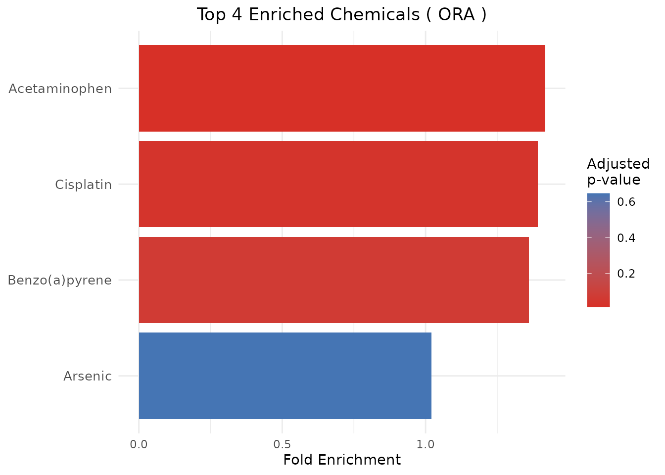
# ORA dot plot (size = gene count, color = adjusted p-value)
plot_CTD(ora_results, type = "dot", n = 10)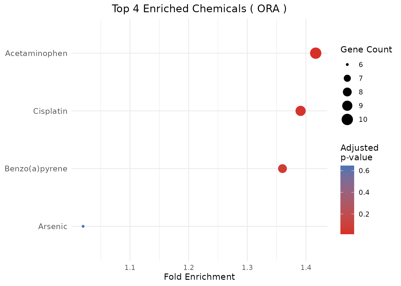
# CAMERA bar plot: x-axis = -log10(padj), fill = Direction
plot_CTD(camera_results, type = "bar")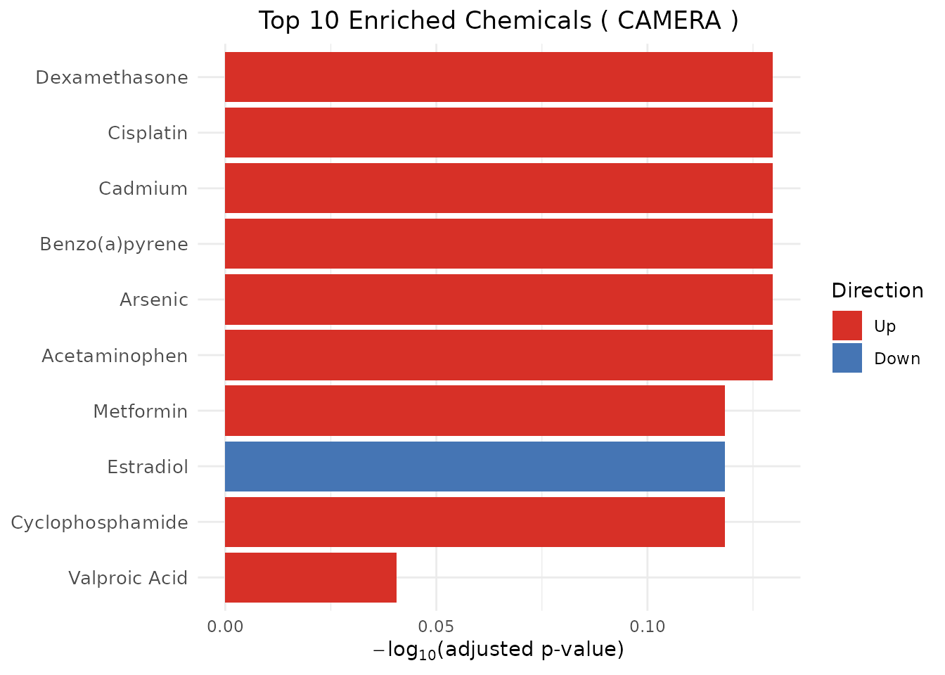
# GSVA heatmap: top-variance chemicals across samples
plot_CTD(gsva_scores)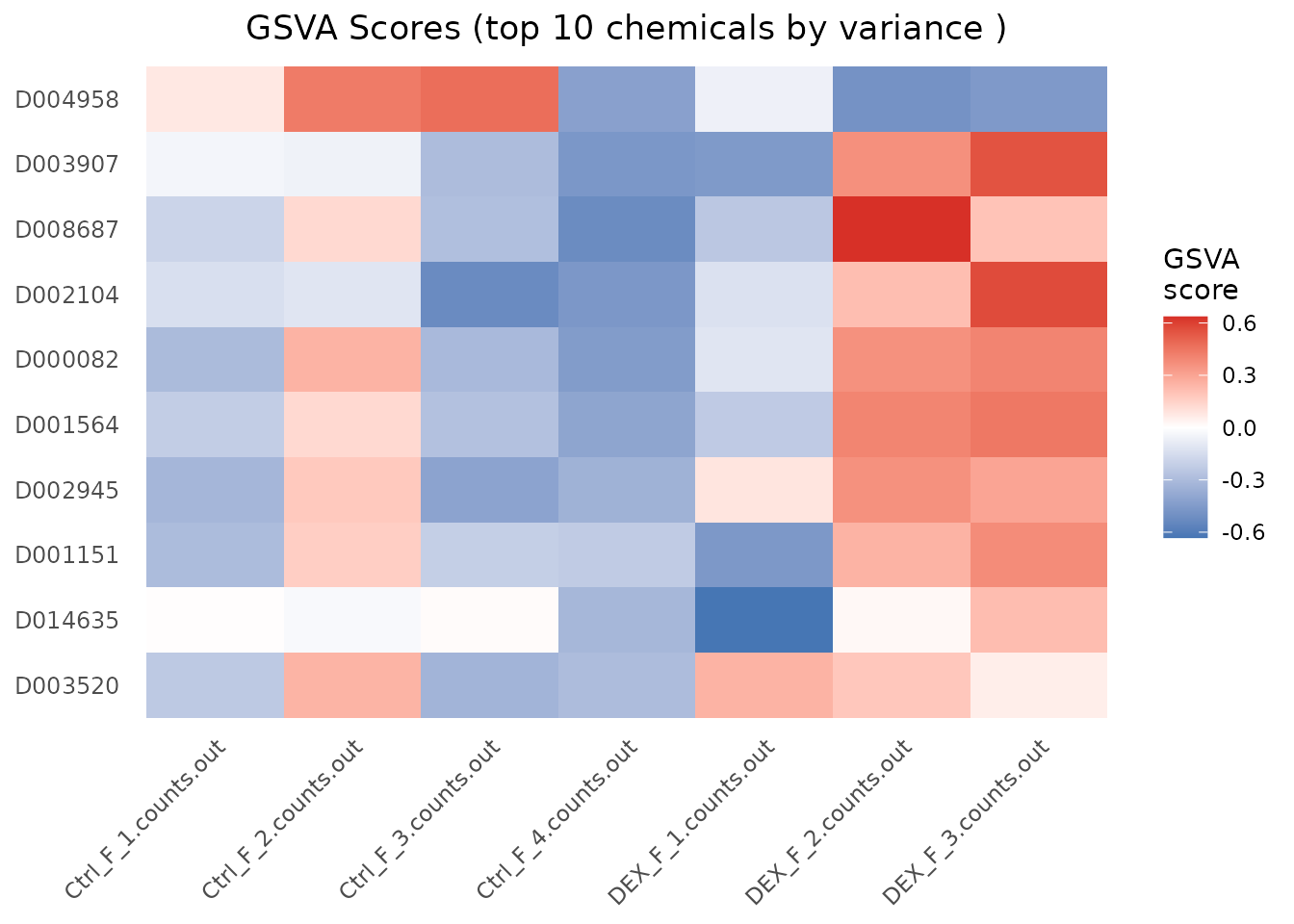
Adjusting for multiple testing
By default, enrichment_CTD() uses the Benjamini-Hochberg
("BH") method for p-value adjustment. You can change this
via the pAdjustMethod parameter:
# Bonferroni correction (more conservative)
ora_bonf <- enrichment_CTD(genes, method = "ORA",
    pAdjustMethod = "bonferroni")
#> Warning in merge.data.frame(res, chemicals_meta, by = "ChemicalID", all.x =
#> TRUE): column name 'FoldEnrichment' is duplicated in the result

# No adjustment
ora_raw <- enrichment_CTD(genes, method = "ORA",
    pAdjustMethod = "none")
#> Warning in merge.data.frame(res, chemicals_meta, by = "ChemicalID", all.x =
#> TRUE): column name 'FoldEnrichment' is duplicated in the result

# Compare the adjusted p-value of the top hit
data.frame(
    method = c("BH (default)", "bonferroni", "none"),
    top_padj = c(min(ora_results$padj),
        min(ora_bonf$padj), min(ora_raw$padj))
)
#> Warning in min(ora_results$padj): no non-missing arguments to min; returning
#> Inf
#> Warning in min(ora_bonf$padj): no non-missing arguments to min; returning Inf
#> Warning in min(ora_raw$padj): no non-missing arguments to min; returning Inf
#>         method top_padj
#> 1 BH (default)      Inf
#> 2   bonferroni      Inf
#> 3         none      Inf
Available methods: "BH" (default),
"bonferroni", "fdr" (alias for BH),
"none".
Gene set size filters and background universe
Each method applies a gene set size filter and defines a background universe, but the degree of user control differs:
| Method | Size filter | Configurable | Background universe | Configurable |
|---|---|---|---|---|
| ORA |
minGSSize / maxGSSize
|
✓ | All genes in TERM2GENE (default) or user-supplied
universe
|
✓ |
| GSEA |
minSize / maxSize
|
✓ | No universe concept — uses the full ranked list | — |
| CAMERA | ≥ 2 genes (hard-coded) | ✗ | rownames(expr) |
implicit |
| GSVA |
minSize / maxSize
|
✓ | rownames(expr) |
implicit |
ORA, GSEA, and GSVA accept size-filter arguments via
..., which are forwarded to the underlying engine. CAMERA’s
minimum of 2 genes is hard-coded and cannot be changed.
# ORA: restrict background to expressed genes and apply size filters
ora_expressed <- enrichment_CTD(
    genes, method = "ORA",
    universe   = c(genes$EntrezID, "7422", "836"),  # expressed genes
    minGSSize  = 3,
    maxGSSize  = 300
)

# GSEA: filter gene sets by size
gsea_filtered <- enrichment_CTD(
    genes, method = "GSEA",
    minSize = 3,
    maxSize = 300
)
#> Warning: GSEA: no 'stat' column found in input. Falling back to -log10(second
#> column) for ranking, which loses directionality and may produce ties at
#> non-significant genes. Add a signed ranking statistic (e.g. the moderated
#> t-statistic from limma::eBayes()) as a column named 'stat' to suppress this
#> warning.
#> Warning in prepareStats(stats, scoreType, gseaParam): All values in the stats
#> vector are greater than zero and scoreType is "std", maybe you should switch to
#> scoreType = "pos".
Setting universe in ORA to the full list of genes
measured in your experiment (rather than the default of all
CTD-annotated genes) is strongly recommended: it avoids inflated
fold-enrichment estimates that arise when the background is larger than
the actual measurement space.
Choosing among the four methods
| Aspect | ORA | GSEA | CAMERA | GSVA |
|---|---|---|---|---|
| Input | Gene list | Ranked gene list | Expression matrix + design + contrast | Expression matrix |
| Question | Over-represented? | Cluster at extremes? | Stronger signal than rest of transcriptome (correlation-corrected)? | Per-sample chemical score |
| Output | Ranked chemicals (data.frame) | Ranked chemicals (data.frame) | Ranked chemicals (data.frame) | Chemical x sample score matrix |
| Best for | DEG lists | Exploratory, ranked | Multi-sample DE experiments, co-regulated gene sets | Patient stratification, downstream tests, heatmaps |
Use ORA when you have a well-defined gene list above a significance threshold; GSEA to leverage the full ranking without a cutoff; CAMERA when you have a proper multi-sample design and want to control the inflated false-positive rate that ORA/GSEA exhibit on strongly co-regulated gene sets; GSVA when you want a per-sample score to feed into downstream analyses (clustering, survival, correlation with phenotypes).
Updating the CTD data
CTD releases updated data periodically. To update:
- Download the latest
CTD_chem_gene_ixns.csv.gzfrom https://ctdbase.org/reports/CTD_chem_gene_ixns.csv.gz. - Decompress and re-run
import_CTD()– existing cache files are overwritten.
import_CTD("~/Downloads/CTD_chem_gene_ixns.csv")Session info
sessionInfo()
#> R version 4.6.1 (2026-06-24)
#> Platform: x86_64-pc-linux-gnu
#> Running under: Ubuntu 24.04.4 LTS
#>
#> Matrix products: default
#> BLAS:   /usr/lib/x86_64-linux-gnu/openblas-pthread/libblas.so.3
#> LAPACK: /usr/lib/x86_64-linux-gnu/openblas-pthread/libopenblasp-r0.3.26.so;  LAPACK version 3.12.0
#>
#> locale:
#>  [1] LC_CTYPE=C.UTF-8       LC_NUMERIC=C           LC_TIME=C.UTF-8
#>  [4] LC_COLLATE=C.UTF-8     LC_MONETARY=C.UTF-8    LC_MESSAGES=C.UTF-8
#>  [7] LC_PAPER=C.UTF-8       LC_NAME=C              LC_ADDRESS=C
#> [10] LC_TELEPHONE=C         LC_MEASUREMENT=C.UTF-8 LC_IDENTIFICATION=C
#>
#> time zone: UTC
#> tzcode source: system (glibc)
#>
#> attached base packages:
#> [1] stats     graphics  grDevices utils     datasets  methods   base
#>
#> other attached packages:
#> [1] ctdR_0.99.6      BiocStyle_2.40.0
#>
#> loaded via a namespace (and not attached):
#>   [1] splines_4.6.1               ggplotify_0.1.3
#>   [3] tibble_3.3.1                polyclip_1.10-7
#>   [5] enrichit_0.2.0              graph_1.90.0
#>   [7] XML_3.99-0.23               lifecycle_1.0.5
#>   [9] httr2_1.2.3                 processx_3.9.0
#>  [11] lattice_0.22-9              vroom_1.7.1
#>  [13] MASS_7.3-65                 magrittr_2.0.5
#>  [15] limma_3.68.4                sass_0.4.10
#>  [17] rmarkdown_2.31              jquerylib_0.1.4
#>  [19] yaml_2.3.12                 otel_0.2.0
#>  [21] ggtangle_0.1.2              cowplot_1.2.0
#>  [23] DBI_1.3.0                   RColorBrewer_1.1-3
#>  [25] abind_1.4-8                 GenomicRanges_1.64.0
#>  [27] purrr_1.2.2                 BiocGenerics_0.58.1
#>  [29] yulab.utils_0.2.4           tweenr_2.0.3
#>  [31] rappdirs_0.3.4              aisdk_1.4.12
#>  [33] gdtools_0.5.1               IRanges_2.46.0
#>  [35] S4Vectors_0.50.1            enrichplot_1.32.0
#>  [37] ggrepel_0.9.8               irlba_2.3.7
#>  [39] tidytree_0.4.8              GSVA_2.6.2
#>  [41] annotate_1.90.0             pkgdown_2.2.0
#>  [43] DelayedMatrixStats_1.34.0   codetools_0.2-20
#>  [45] DelayedArray_0.38.2         DOSE_4.6.0
#>  [47] ggforce_0.5.0               tidyselect_1.2.1
#>  [49] aplot_0.3.0                 memuse_4.2-3
#>  [51] farver_2.1.2                ScaledMatrix_1.20.0
#>  [53] matrixStats_1.5.0           stats4_4.6.1
#>  [55] Seqinfo_1.2.0               jsonlite_2.0.0
#>  [57] systemfonts_1.3.2           tools_4.6.1
#>  [59] ggnewscale_0.5.2            treeio_1.36.1
#>  [61] ragg_1.5.2                  Rcpp_1.1.2
#>  [63] glue_1.8.1                  SparseArray_1.12.2
#>  [65] xfun_0.59                   qvalue_2.44.0
#>  [67] MatrixGenerics_1.24.0       dplyr_1.2.1
#>  [69] HDF5Array_1.40.0            withr_3.0.3
#>  [71] BiocManager_1.30.27         fastmap_1.2.0
#>  [73] rhdf5filters_1.24.0         callr_3.8.0
#>  [75] digest_0.6.39               rsvd_1.0.5
#>  [77] R6_2.6.1                    gridGraphics_0.5-1
#>  [79] textshaping_1.0.5           GO.db_3.23.1
#>  [81] RSQLite_3.53.3              h5mread_1.4.0
#>  [83] tidyr_1.3.2                 generics_0.1.4
#>  [85] fontLiberation_0.1.0        data.table_1.18.4
#>  [87] httr_1.4.8                  htmlwidgets_1.6.4
#>  [89] S4Arrays_1.12.0             scatterpie_0.2.6
#>  [91] pkgconfig_2.0.3             gtable_0.3.6
#>  [93] blob_1.3.0                  S7_0.2.2
#>  [95] SingleCellExperiment_1.34.0 XVector_0.52.0
#>  [97] clusterProfiler_4.20.0      htmltools_0.5.9
#>  [99] fontBitstreamVera_0.1.1     bookdown_0.47
#> [101] fgsea_1.38.0                GSEABase_1.74.0
#> [103] scales_1.4.0                Biobase_2.72.0
#> [105] png_0.1-9                   SpatialExperiment_1.22.0
#> [107] ggfun_0.2.1                 knitr_1.51
#> [109] tzdb_0.5.0                  reshape2_1.4.5
#> [111] rjson_0.2.23                nlme_3.1-169
#> [113] org.Hs.eg.db_3.23.1         cachem_1.1.0
#> [115] rhdf5_2.56.0                stringr_1.6.0
#> [117] parallel_4.6.1              AnnotationDbi_1.74.0
#> [119] desc_1.4.3                  pillar_1.11.1
#> [121] grid_4.6.1                  vctrs_0.7.3
#> [123] BiocSingular_1.28.0         tidydr_0.0.6
#> [125] beachmat_2.28.0             xtable_1.8-8
#> [127] cluster_2.1.8.2             evaluate_1.0.5
#> [129] readr_2.2.0                 magick_2.9.1
#> [131] cli_3.6.6                   compiler_4.6.1
#> [133] rlang_1.3.0                 crayon_1.5.3
#> [135] labeling_0.4.3              ps_1.9.3
#> [137] plyr_1.8.9                  fs_2.1.0
#> [139] ggiraph_0.9.6               stringi_1.8.7
#> [141] BiocParallel_1.46.0         Biostrings_2.80.1
#> [143] lazyeval_0.2.3              GOSemSim_2.38.3
#> [145] fontquiver_0.2.1            Matrix_1.7-5
#> [147] hms_1.1.4                   patchwork_1.3.2
#> [149] sparseMatrixStats_1.24.0    bit64_4.8.2
#> [151] ggplot2_4.0.3               Rhdf5lib_2.0.0
#> [153] KEGGREST_1.52.2             statmod_1.5.2
#> [155] SummarizedExperiment_1.42.0 igraph_2.3.3
#> [157] memoise_2.0.1               bslib_0.11.0
#> [159] ggtree_4.2.0                fastmatch_1.1-8
#> [161] bit_4.6.0                   ape_5.8-1
#> [163] gson_0.2.0